

How To Change Units In A Zemax Spot Diagram
ZEMAX RAY-TRACING EXECRISE NOTES FROM OPTICAL CONSTRUCTION Grade
RT0
Standard Spot Diagram
Clicking in the "Standard Spot Diagram" icon under the "Rays & Spot" icon in the Paradigm Quality grouping under the "Analyze" tab.
You will in this spot diagram see the position of a number of rays originating from the object at the position of the image airplane. Information about the size of the spot is given, both in terms of an RMS radius and a GEO radius in the lower office of the plot. The GEO radius is the radius of a circumvolve in the epitome plane in which all rays autumn. The RMS radius is the root-mean-foursquare value of the radius of the positions the rays intercept in the prototype plane. The latter ane is the virtually relevant. Yet, it can be worth to note that since a ray tracing program only calculates the fate of certain rays, the values of these ii indicators (the RMS and the GEO radii) depend on how many rays the plan considers and in which "design" they are sent out. There is a standard set up of ray patterns and number of rays that the program uses, but one can also chose other sets. You can toggle between three such patterns in the Setting window, which yous open by clicking on the small downwards arrow in the upper left corner of the window of the Spot Diagram. Alter between, "Squared", "Hexapolar", and "Dithered", and meet the effect of this. You can also increase the number of rays. For a uncomplicated system like this, the extra time it takes to summate more than rays than the predetermined value of half-dozen is negligible. Therefore, apply to some larger value, e.g. 24, and see the event. Use "Dithered" and a ray density of 24. What is the RMS size of this spot (you should get an RMS spot size betwixt 200 and 400 µm, if non, redo)
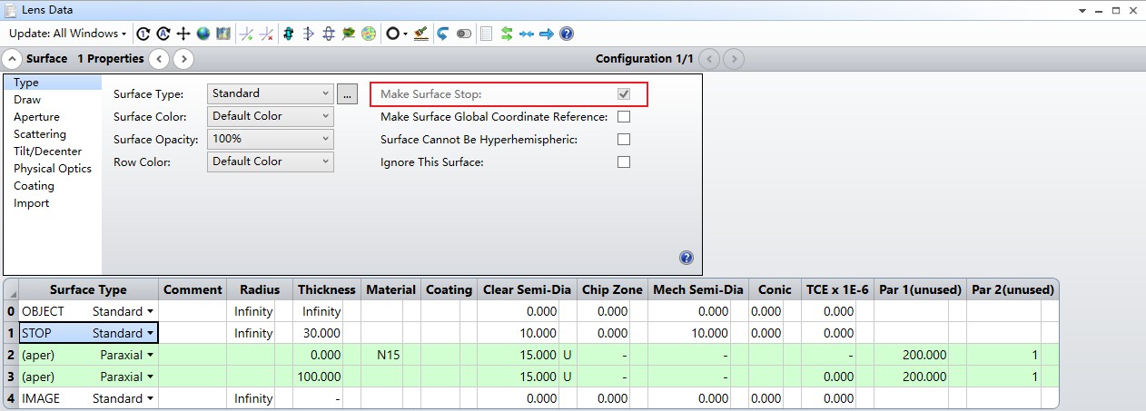
"Solve" routine
There is besides another way of finding the paraxial position of the image (instead of using the optimization routine), namely to use a "Solve" routine. To utilise the "Solve" routine, double-click on the minor foursquare box of the cell y'all just optimized (the thickness cell of row two) and, instead of using "Variable", chose "Marginal Ray Tiptop". This solve-routine will aid the program to find the value of the lens-to-image altitude that forces the marginal ray (the marginal ray is the ray that originates from the optical axis and passes the aperture terminate/archway pupil at a given height/pupil zone, in general at the rim of the aperture stop/entrance pupil) to arrive at a height given past the "Height" value in the image aeroplane. We want to discover the paraxial focus. Hence, the ray height should be specified to 0 (which is the default value).
Next to specify is which ray should exist considered. You specify this by specifying a "Pupil Zone" value. We know now that the paraxial focus is the position for which rays with a almost zilch bending focus to 1 spot (all higher order terms get negligible). The "Pupil Zone" value refers to the (normalized) peak of the beam in the entrance aperture (the Terminate surface) of the system. We get rays with 0 angles, and hence the position of the paraxial focus, by specifying the Educatee Zone" value to 0. Therefore, run "Marginal Ray Height" with zeros for both the "Height" and the "Pupil Zone" values.
RAY- RACING USING ARAXIAL SURFACES
The ZEMAX program has also a possibility to use not-spherical surfaces (as for example, adding a pocket-size conical beliefs to the spherical shape that volition compensate for many types of aberrations).
But, it has likewise the sometimes useful feature of introducing completely aberration-gratis surfaces (i.due east. a surface that exactly follows theparaxial theory). These are called paraxial surfaces.
RT1
Create a Lens Data editor that describes the state of affairs. Start by making a lens made out of
two lens surfaces, each of them of paraxial type (and each having one-half the refractive ability, i.e., twice the actual focal length, i.eastward. forty mm), but, with no distance in between. This is
convenient when comparisons with finite thickness lenses are going to be washed afterwards on. Select an "Archway Aperture Bore" of 10 mm nether the "Aperture" tab of the System
EXPLORER. Place the image plane at a and then far capricious position behind the lens, e.thou. at 100 mm. For display purposes, you can make the lens larger than the minimum size. Give the lens, for simplicity, a semi-bore of 8 mm.
run the optimization procedure (practice non forget to outset with the "Optimization Wizard" icon in the Automatic Optimization grouping under the "Optimize" tab, and use Type: "RMS", Criteria "Spot Radius", and Reference "Principal Ray" equally be-fore, and use iv rings, before you run "Optimize!" in the Automatic Optimization group under the "Optimize" tab) and discover out where the image plane is localized. Look also at the Layout.
Decide the transverse magnification
In order to determine the transverse magnification of the arrangement, y'all need to place another object at a certain altitude from the optical axis. Open the "Fields" tab in the Organization EXPLORER. The blazon of field chosen under "Settings"should exist "Object Acme". If not set up, change to this. By default, you accept one field point set (termed Field ane). If you open up this tab, you lot will come across that this field point is at ten = 0, and y = 0, and that it has a weight of 1. Now y'all need to create some other field point. Open the "Add together Field" tab and set this at x = 0, and y = ten, with a weight of 1. Note that you have to click on the Enable box, be able to set this field indicate.
Retrieve this for the futurity. Every time you alter the number of field points (or the number of wavelengths, see coming exercises) you need to open and run the Merit Function Editor once again.
the actual position of the rays from the uppermost part of the object can, for ex-aplenty, exist found by invoking the "Standard Spot Diagram" icon nether the "Rays & Spot" icon in the Image Quality group nether the "Analyze" tab. You lot should be able to read the middle position of the beams both at the object and the image aeroplane. The ratio should requite you the transverse magnification. Which transverse magnification does this organisation have?
Fixed L = SIM + SOB
In this case yous need to optimize an intermediate position (i.eastward. that of the lens) while property the object-to-epitome altitude stock-still. You lot can accomplish this by double clicking on the Thicknesscell of the last lens surface and choose "Position" instead of "Fixed" or "Variable" that we take used before. Yous can hither decide the position from some other given surface. Choose "From Surface:" "0" and "Length:" "160". This implies that the prototype plane always will be positioned 160 mm behind the object plane. Hence, y'all tin can now optimize the position of the lens as yous want. Change the Thickness cell of the uppermost row to "Variable" and then that you tin optimize the position of the lens. A possible starting point (if y'all model your lens as 2 surfaces) could then look like as foll.
Add the magnification constraint
One manner of doing this is to open the merit role(in Wizards and operand)and and then add one more opti-mization status (the magnification constraint). This yous can exercise by calculation one more than line in the merit function. This line should be the beginning line. Click in any of the cells in the DFMS line. Printing "Insert". They yous get a dummy line, with the command BLNK (for Bare) equally the type. You need to commutation this to some more useful command. Click in the small squared box of this cell. Y'all should then get a list of possible optimization operands. These you can use at any time in your ray tracing (you can read near this in the assist files). In this instance, employ PMAG, since this puts a requirement on the paraxial magnification. This magnification nosotros want to lock to -0.5. Therefore, blazon PMAG for the "type" of this operand (in identify of BLNK). You need to give the target value of this, which thus is -0.5. Type this in the target cavalcade. Then you need to give it a weight. Give information technology a weight of ane (which is a standard value). Now when you run the optimization, the program will both try to minimize the spot size in the image plane (or the aberrations) but also try to accomplish a arrangement with a paraxial magnification of -0.5. Run the optimization and make up one's mind the focal length and the lens position.
RT2
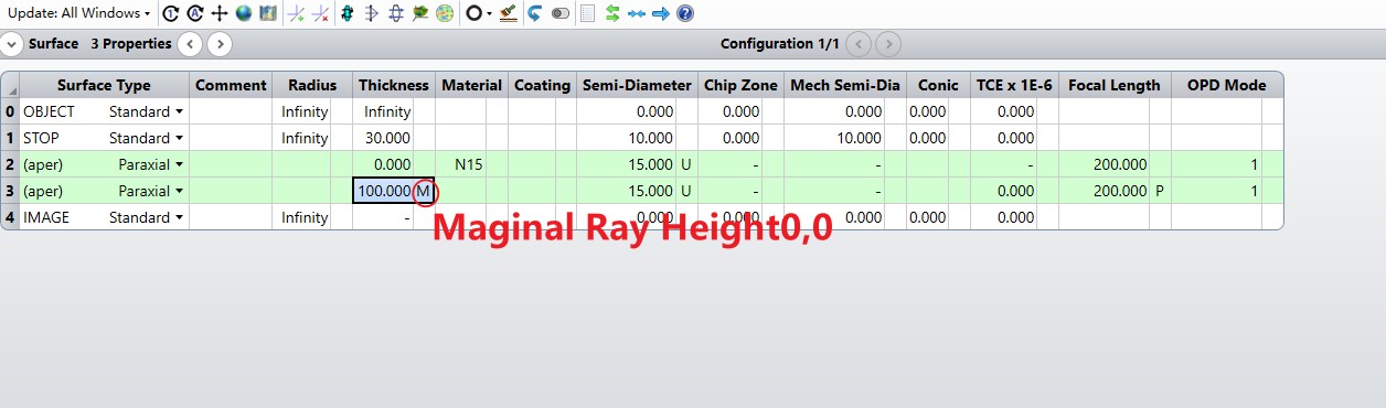
Recall that in order to go the focal length of such a organisation (which is a parax-ial quantity), you accept to expect at rays that get close to the optical centrality. This yous tin can practise either by using the optimization routine for the focal length (with the radii of curvature of the first surface equally a variable, with the second surface having the same radius of curvature but with opposite sign, which tin exist done by the "Pick up" routine, with a fixed value for the distance between the terminal surface and the paradigm plane, and with a very small entrance pupil bore) or by using the Solve routine for the marginal ray height ("Marginal Ray Superlative", 0,0) and manually trying various radii
Creating a parallel pencil of rays
let the object accept an in-finite distance to the showtime surface, which also is the "Aperture Stop" (also called the "Surface Stop" in ZEMAX). If yous desire to run into some parts of the parallel rays falling in on your lens arrangement (in the Layout window) you can add an extra non-refractive dummy surface in front of the lens. This non-refractive surface, which can serve as the archway pupil, should non refract the rays. Hence, it should exist fol-lowed by only air (no glass textile). Information technology should, notwithstanding, take a certain distance to the lens. This distance can be quite arbitrary (since parallel lite rays are emerg-ing from the surface) so equally to create a overnice layout.
Insert therefore a new surface straight later on the object surface. (Click in any cell of surface 1 and press the "Insert" fundamental on the keyboard.) Type a suitable number for its thickness in the"Thickness"column. Any number in the range ten to 50 will suffice. Brand sure that the distance from the object to the offset "dummy" surface is infinite. Allow this time the dummy surface be the "Aperture Stop". You do this by double clicking in the first cell of the row, which reads "ane", (or by marking any cell of row 1 and and so opening the "Settings" window, which yous do by pressing the arrow that points down enclosed in a circle (i.eastward. ) and click in the box for the "Make Surface Finish". You will discover that the surface end has changed from the outset surface of the lens to this new fictitious surface. When you look in the Layout window, brand sure yous plot the optical system from surface 1 to surface 4 (come across the "Settings" window). Nosotros will come up back to the importance of the" Aperture Finish"in afterwards Ray Tracing exercises.
One why to find this is to use the optimization routine you used in a previous Ray Tracing exer-cise, another is "Marginal Ray Superlative" solve (for the latter, double-click on the pocket-sized square box of the thickness prison cell of the terminal surface of the lens and cull "Marginal Ray Tiptop")
Prepare Surface Stop
Make sure that the lens is the "Surface Cease". (If not, double-click in the first cell of the offset surface of the lens, i.east. the jail cell that reads "Paraxial",and then click in the "Brand Surface Stop" box.
Optimize the arrangement
When you optimize the system, do not forget to beginning with the "Optimization Wiz-ard" icon in the Automated Optimization group under the "Optimize" tab, and apply Blazon: "RMS", Criteria "Spot Radius", and Reference "Chief Ray" as earlier, and use 4 rings, before you lot run "Optimize!" in the Automatic Optimization group under the "Optimize" tab
Report
You can find data virtually the positions of the principal planes of an optical system in "Prescription data", which you detect under the nether the "Re-port" icon in the Reports group under the "Analyze" tab. and thereby bank check that the equation you derived above is correct.
Case
Open up the "Cooke 40 degree field" lens (1 of the instance files that are supplied with the program, can be found under Zemax\sample\sequential\objectives)1 and look at the layout window. This organisation shows the bones design of a real Cooke .triplet. One positive lens, one negative lens (made of another glass material so as to minimize chromatic aberrations, something you volition look closer to in a comingray tracing exercise) followed by one positive lens finally. You lot can see how lite from three different angels (from far away, e.yard. infinity) propagate through the arrangement. Please hold this system in your heed when you are working with the sim-plified paraxial lenses in the practice beneath (so you do not lose grip of the reality).
RT4
Specify that the wavelength of the low-cal
Specify that the wavelength of the light is 587.562 nm. This you practice by opening the "Wavelength"tab in the Arrangement EXPLORERand so, nether "Settings" and"Preset", select "d(0.587)". When you have selected this every bit your chief wave-length, press the button "Select Preset" to execute this choice. You can encounter that you take selected this wavelength as your primary wavelength if the text in the next tab "Wavelength 1 (0,xxx μm, Weight = i,000)" displays this wavelength, i.e. if it reads "Wavelength 1 (0,588 μm, Weight = 1,000)".
Cloth catalogue
The reason for this item wavelength to be of special importance is that information technology cor-responds to a yellowish line in the spectrum from helium (at 587.5618 nm). The in-dex of refraction at this wavelength is commonly abbreviated dn. Find out what the actual alphabetize of refraction of BK7 is at this wavelength, i.east. decide the dn - value. (There is an extensive catalogue with many types of spectacles, termed "mate-rial catalogue", incorporated into the program that can give you a lot of useful in-germination. Call back that BK7 is a Schott glass.)
Find a particular glass
he easiest way to find a particular glass in this catalogue is to blazon BK7 in the Material column in the Lens Data editor and and so mark the name of the glass exist-fore you open the material catalogue. It and then opens straight with information virtually this item blazon of glass at this particular wavelength, i.e. with info near n_d. alternatively, if you type BK7 in the Material column in theLens Data editor, you can also discover its index of refraction for the wavelength used (thus non only at 587.5618 nm) in "Prescription information", which you lot discover under the nether the "Re-ports" icon in the Reports group nether the "Analyze" tab. Look about half down the document. Check that you can observe the value of the index of refraction at both places.
The (RMS) spot size of the focus
The (RMS) spot size of this focus (look in the "Standard Spot Diagram"icon under the "Rays & Spot" icon in the Image Quality group under the "Ana-lyze" tab and apply "Dithered" as "Pattern" under "Settings" and a ray density of 24)?
Selecting "F, d, C (visible)"
Expand now the number of wavelengths you are using to 3. In the "Wavelength" tab in the SYSTEM EXPLORER you should use 486.i nm as wavelength number 1, 587.half-dozen nm every bit wavelength number 2 and 656.three nm as wavelength number 3 (the yel-low helium line and the blueish and cherry hydrogen Fraunhofer lines). Make the 0.5876 μm wavelength the "master" one. Annotation that y'all can go all these iii moving ridge-lengths directly by selecting "F, d, C (visible)" nether "Settings" and "Preset". When y'all accept pressed"Select Preset" yous should get iii lines(tabs) of wave-lengths below the "Settings" tab reading"Wavelength 1 (0,486 μm, Weight = i,000)",
"Wavelength ii (0,588 μm, Weight = i,000)",
"Wavelength iii (0,656 μm, Weight = 1,000)"
Select all wavelength
there is a "Wavelength" box in the upper right about corner in which yous tin can specify which wavelengths y'all want to study. Cull "All". You lot demand also to choose "Wave #" in the "Color Rays By:"box. Do the same with the "Spot Diagram" window (and utilize over again "Dithered"and a "Ray Density" of 24). You lot are at present ready to see what happens with all the light beams in the system.
Update all widows
(double click in them or use the fast red button with two curly arrows in theQUICK ACCESS TOOLBAR).
Dealing with chromatic aberration.
There are two different windows that are of detail utilize when dealing with chromatic aberration. The first ane is called "Focal Shift" and tin be opened by invoking the "Chro-matic Focal Shift" icon nether the "Aberrations" icon in the Image Quality grouping under the "Clarify" tab. This window shows you the shift in focal length every bit a function of wavelength.
The other useful window is the "Through Focus Spot Diagram" and can be opened by invoking the" Through Focus Spot Diagram" icon under the "Rays & Spot" icon in the Epitome Quality group nether the "Clarify" tab. This window shows you five different spot diagrams. Adjusting some parameters under "Gear up-tings" (the arrow that points down enclosed in a circumvolve, i.e. the ) will requite you a nice result. Choose a "Ray Density" effectually 5 - 10 (depending on your monitor), "Delta Focus" to 500 (μm), do not select "Use Symbols", use "Pattern:" "Dith-ered", and make sure that "Wavelength" is ready to "All". Depending on your moni-tor, yous tin can play around with the line thickness, it is often easiest to run into this if you select the "thin" or "thinnest" line thickness (change "standard" to "thin" or "thin-nest").
What you will come across is how the spot diagrams await like in focus, as well as 500 and yard μm in front of and behind the focus. Every bit you come across in this case, the focus of the green wavelength (i.east. the one at 587 nm, the center one in wavelength) is shut to the selected image plane (i.e. in focus), the blueish wavelength (486 nm) has a fo-cus about ane mm in front end of this focus while the red ane (656 nm) has its focus near half a millimeter backside the selected focus. This is a pictorial illustration of what the "Through Focus Spot Diagram" shows.
Constructive focal length by using marginal ray bending
Select now somewhat more suitable thicknesses of the lenses: 3 mm for the kickoff one and 2 mm for the 2d 1. The actual focal length will then change. Reop-timize the optical arrangement so that you go a focal length of exactly 100 mm by let-ting both the kickoff radius and the distance between the final lens and the epitome airplane be variable, make the starting time lens symmetrical, i.e. 11RR′= − (by a pick up of the kickoff surface), let the lenses exist cemented, i.e. 21RR′=, and use a "Marginal Ray Bending" solve of the radius of the last lens surface of -0.1. The "Marginal Ray Angle" solve is a useful manner of getting a certain effective focal length. A "Mar-ginal Ray Bending" solve of the radius of the terminal lens surface of -0.1 should give you an constructive focal length of 100 mm. Spend some time thinking about whythis is the case. What does a marginal ray angle of -0.1 imply?
RT5
Standard Spot Diagram
The GEO radius, given in the lower office of the plot, gives the radius inside which all the rays are collected. Hence, the GEO radius gives information about the dis-tance to the ray that is uttermost from the central reference point. This radius thus corresponds to the maximum ray aberrations Yε and Xε defined in the course material.The RMS radius, on the other hand, gives a root-hateful-foursquare value of the radius of all the rays. The RMS radius is often a more useful and representative entity since it gives a weighted distribution of the rays.
Through Focus Spot Diagram"
The "Through Focus Spot Diagram" shows you the spot diagram from a number of rays emerging from one (or a selected number of) single point in the object plane not simply in the image plane but also at a few planes in shut proximity to the paradigm plane. This carte du jour is peculiarly useful in systems where some rays will fo-cus in front of the chosen image plane while others focus slightly behind, every bit oc-curs for "Chromatic Aberrations" as well as a few of the monochromatic aberra-tions, e.g. "Spherical Aberration" and "Curvature of Field".You volition address these in detail in future problem sets. When you invoke this window for the unmarried lens, you will detect two rows with five spot diagrams in each. Each spot diagram in each row southward calculated for a specific position with respect to the chosen paradigm plane. The centre i is exactly at the position of the image plane. The other ones are the spot diagrams every bit they wait in front or behind the image plane. The two rows represent to the two fields. In the "Settings" menu in that location is a box for specifying the shift in position between each of these diagrams ("Delta Focus") in units of μm. Select 1000 μm and make sure you are looking at the single lens. Select "Dithered" and a suitable "Ray Density" besides in the "Options" window (12 is adequately OK). Yous can switch exist-tween to "Utilise Symbols" and not to "Use Symbols", and to apply "All" or i wavelength at a fourth dimension in the "Wavelength" box to meet what y'all think is best for your detail application. Starting time with the unmarried lens.
Enclosed Energy
The programme gives the user also the possibility to investigate the corporeality (or frac-tion) of rays in a fan that hits the image plane inside a certain radius from the spot. This is referred to as "Enclosed (or Encircled) Energy". Under the Image Quality grouping under the "Analyze" tab y'all can find the "Enclosed Energy" icon. Under this, you can find few different types of "Enclosed Energy" diagram of which 2 are "Diffraction" and "Geometric.
Optical Path
The plan can also display cuts through the "Wave Map", so called "OPD Fans" ("Wave Aberration Sections "in the course fabric) or "OPD" diagrams, where "OPD" stands for "Optical Path Difference". This tin be opened by invok-ing the "Optical Path" control under the " "Aberrations" icon in the Image Quality group under the "Analyze" tab. They will give yous information about the optical path difference forth the tangential and sagittal cuts at the exit student (the two orthogonal directions of the "Wavefront Map"). If more than one wavelength is used, one curve for each wavelength will be dis-played. Expect at the "OPD Fans" for the two lenses. Await not merely at the shapes of the curves for the ii optical systems; pay besides attending to the maximum scales (which sometimes can be more important than the bodily shapes).
Ray Fan
The program can likewise display cuts through the "Spot Diagram" display. The "Ray Fan" window tin can be opened by invoking the "Ray Aberration" command either under the "Rays & Spot" icon or the "Aberrations" icon in the Prototype Quality group under the "Analyze" tab. This window shows plots of the ray aberration (defined as the deviation between the actual paradigm point and the prototype point of the chief ray in the image aeroplane) as a function of the height of the leave educatee.The "Ray Fan" curves are also the derivatives of the OPD curves discussed above. You get three curves in each diagram (corresponding to the three wave-lengths), ane diagram for each plane (tangential and sagittal) and ane pair of dia-grams for each field (bundle of ray direction). Compare the "OPD" curves with the "Ray Fans" and make sure you understand how they are related.
Field Curvature and Distortion
The "Field Curvature" and "Baloney" aberrations can be display past the com-bined "Field Curvature and Distortion" command. This command can exist found under the "Aberrations" icon in the Image Quality grouping under the "Analyze"tab
RT6
OPD Fans
The programme can also display cuts through the "Wave Map", so called "OPD Fans" ("Wave Aberration Sections "in the course material) or "OPD" diagrams, where "OPD" stands for "Optical Path Departure". This can exist opened by invok-ing the "Optical Path" command under the " "Aberrations" icon in the Image Quality grouping under the "Analyze" tab. They will requite you information most the optical path difference forth the tangential and sagittal cuts at the exit pupil (the ii orthogonal directions of the "Wavefront Map").
RT8
Effective Focal Length)
When you optimize, e'er use the default sequential merit function with RMS spot radius referenced to the chief ray. To brand systems with the same constructive focal length, add the operand EFFL (Effective Focal Length) with target 105 on the start line in the merit function editor (make a new line earlier the DMFS line and blazon EFFL in its commencement box). Employ a weight of 1 for the EFFL command.
Prescription data
or every lens that you blueprint, make data sheets that include the most relevant in-germination, which should at least consist of •data about the lenses (radii, types of glass, distances, etc), •a layout, •OPDs, •Ray fans, •spot diagrams, and •a short compilation of the Seidel coefficients. One manner of documenting the information about the lenses (radii, types of glass, distances, etc., i.e. the lens data editor) is to open the "Prescription information", which you find nether the under the "Report" icon in the Reports group nether the "Ana-lyze" tab., since this contains the lens information editor. You can then save this in text format somewhere, and cut the lens data editor from this text file and past it into your text editor. You can practice the aforementioned to recall the Seidel coefficients from the "Seidel coefficient" window, which tin be found under the "Aberrations" icon in the Epitome Quality grouping nether the "Clarify" tab.
Source: https://mercaph.github.io/2020/11/19/ZEMAX-notes/
Posted by: martinhignisfat.blogspot.com
0 Response to "How To Change Units In A Zemax Spot Diagram"
Post a Comment