If The Value Of X Increases By 4, How Does The Value Of M(X- 5) Change?

Understanding The Linear Regression!!!!

Everyone new to the field of data science or automobile learning,often starts their journey by learning the Linear Models of the vast set of Algorithm's available.
So,Permit'southward Start!!!

Content:

What is Linear Regression?
Assumptions of Linear Regression.
Types of Linear Regression?
Agreement Slopes and Intercepts.
How does a linear Regression Work?
What is a Cost Function?
Linear Regression with Slope Descent.
Interpreting the Regression Results.

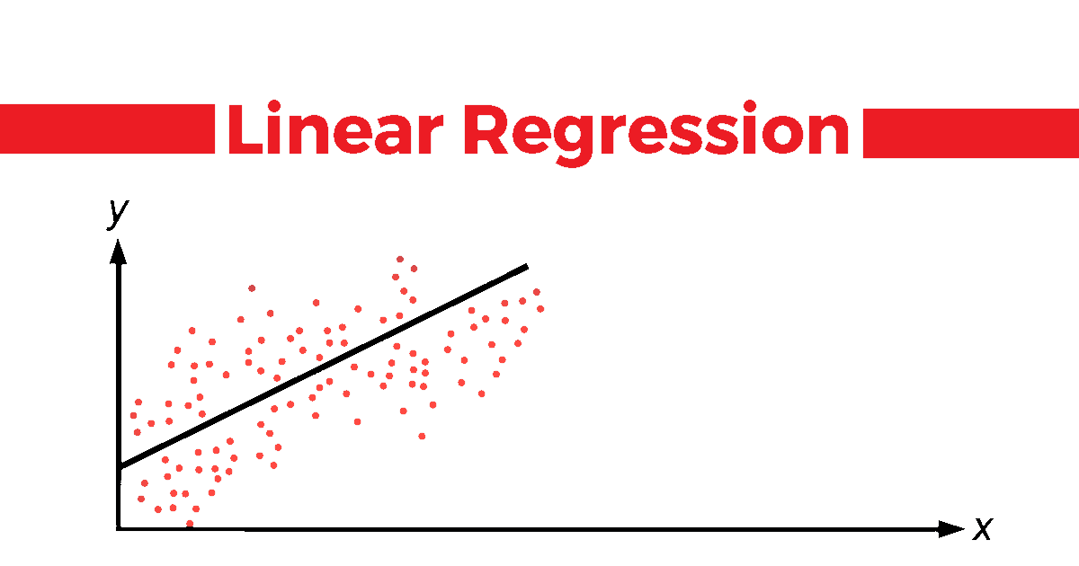
What is Linear Regression?

Linear Regression is a statistical supervised learning technique to predict the quantitative variable by forming a linear human relationship with one or more contained features.
It helps determine:
→ If a independent variable does a good job in predicting the dependent variable.
→ Which contained variable plays a meaning role in predicting the dependent variable.

At present,Every bit you lot know most of the algorithm works with some kind of assumptions.So, Earlier moving on here is the list of assumptions of the Linear Regression.
These assumptions should be kept in mind when performing Linear Regression analysis so that the model performs it's best.

Assumptions of Linear Regression:

The Contained variables should be linearly related to the dependent variables.
This can be examined with the help of several visualization techniques like: Scatter plot or maybe you can apply Heatmap or pairplot(to visualize every features in the data in one item plot).
Every feature in the information is Normally Distributed.
This again can be checked with the help of unlike visualization Techniques,such as Q-Q plot,histogram and much more than.
There should be piffling or no multi-collinearity in the data.
The best way to check the prescence of multi-collinearity is to perform VIF(Variance Inflation Factor).
The mean of the remainder is zero.
A residual is the departure between the observed y-value and the predicted y-value.However, Having residuals closer to zero ways the model is doing nifty.
Residuals obatined should be normally distributed.
This tin can be verified using the Q-Q Plot on the residuals.
Variance of the balance throughout the data should be same.This is known every bit homoscedasticity.
This can be checked with the help of residual vs fitted plot.
There should be petty or no Auto-Correlation is the data.
Machine-Correlation Occurs when the residuals are not independent of each other.This usally takes identify in time series assay.
Yous tin perform Durbin-Watson test or plot ACF plot to check for the autocorrelation.If the value of Durbin-Watson exam is 2 then that means no autocorrelation,If value < 2 and then there is positive correlation and if the value is between >ii to iv then there is negative autocorrelation.

If the features in the dataset are not commonly distributed try out dissimilar transformation techniques to transform the distribution of the features present in the data.

Can you lot say,why these assumptions are needed?

The Gauss-Markov theorem states that if your linear regression model satisfies the first half-dozen classical assumptions, then ordinary to the lowest degree squares ( OLS ) regression produces unbiased estimates that take the smallest variance of all possible linear estimators.

To Read More about the theorem delight go to this link.

Now that few things are Clear allow's movement on!!!

Types of Linear Regression

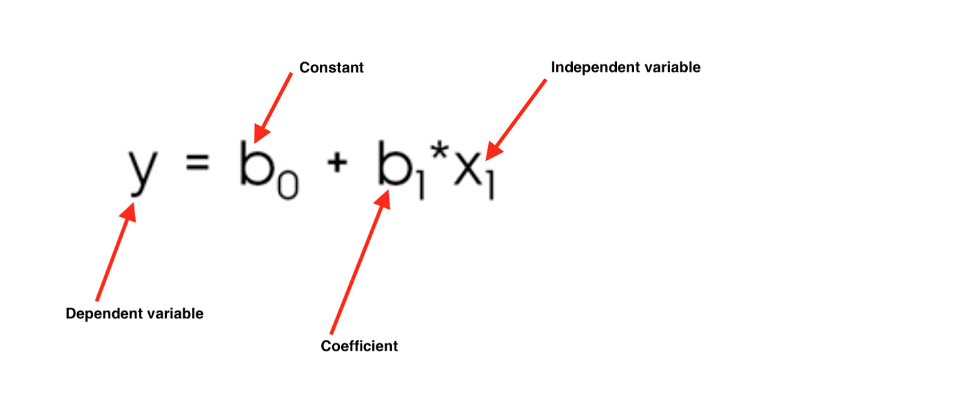
→ Unproblematic Linear Regression:

Elementary Linear Regression helps to notice the linear relationship between 2 continuous variables,One independent and one dependent feature.
Formula can be represented as y=mx+b or,

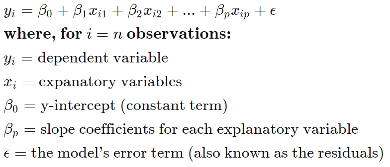
→ Multiple Linear Regression:

Multiple linear Regression is the about mutual grade of linear regression analysis. Equally a predictive analysis, the multiple linear regression is used to explain the relationship between i continuous dependent variable and two or more independent variables.
The independent variables can be continuous or categorical (dummy coded as advisable).
We Ofttimes use Multiple Linear Regression to do whatever kind of predictive analysis equally the data nosotros get has more than ane independent features to it.
Formula can exist represented as Y=mX1+mX2+mX3…+b ,Or

Now that nosotros know different types of linear regression,Let'due south empathise how the slope co-efficients and y-intercept are calculated.

let'due south look below to understand what slope and intercept is.

From,Here on we'll understand the concept with the help of,

Elementary Linear Regression.

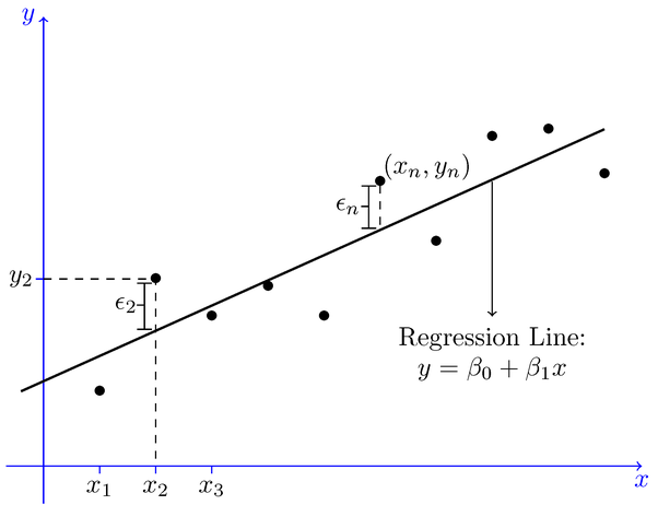
Agreement the Slope and intercept in the linear regression model:

What is a gradient?
In a regression context, the slope is very of import in the equation because it tells you how much you can expect Y to change every bit 10 increases.
It is denoted by m in the formula y = mx+b.

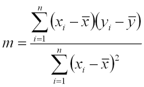
It tin can besides be calculated by the formula,

m = r*(Sy/Sx),
Where r is the correlation co-efficient.
Sy and Sx is the standard difference of ten and y.
And r can be calculated equally

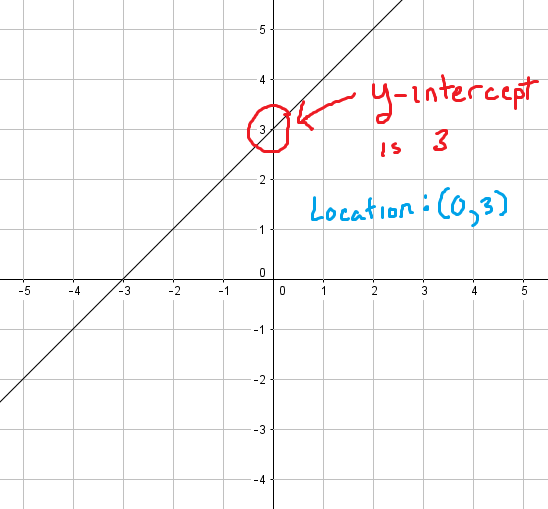
What is Intercept?
The y-intercept is the identify where the regression line y = mx + b crosses the y-axis (where x = 0), and is denoted past b.
Formula to summate the intercept is:

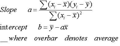
Now,Put this gradient and intercept into the formula (y = mx +b) and their yous have the clarification of the best fit line.

This best fit line will now pass through the data according to the properties of a regression line that is discussed below.Now,What if i tell y'all in that location is nonetheless room to meliorate the best fit line?
As yous know, we desire our model to be the best performing model on unseen data and to exercise so Stochastic Gradient Descent is used to update the values of gradient and intercept,so that we acheive very low toll office of the model.
Don't worry we will wait into it later in this blog.

How does a linear Regression Work?

The whole idea of the linear Regression is to detect the best fit line,which has very low error(cost function).
This line is also called Least Foursquare Regression Line(LSRL).

The line of all-time fit is described with the aid of the formula y=mx+b.
where,m is the Slope and
b is the intercept.

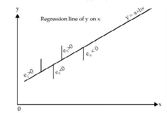
Properties of the Regression line:
1. The line minimizes the sum of squared deviation between the observed values(actual y-value) and the predicted value(ŷ value)
two. The line passes through the hateful of independent and dependent features.

Let's Understand what cost function(error function) is and how slope descent is used to get a very authentic model.

Price Function of Linear Regression

Cost Function is a function that measures the functioning of a Machine Learning model for given data.
Cost Office is basically the calculation of the error between predicted values and expected values and presents it in the form of a single real number.
Many people gets confused between Cost Function and Loss Function,
Well to put this in simple terms Cost Role is the boilerplate of error of north-sample in the data and Loss Part is the error for individual data points.In other words,Loss Role is for 1 training example,Cost Function is the for the entire preparation set.

So,When it'southward clear what cost function is Permit's motility on.

The Cost Part of a linear Regression is taken to be Mean Squared Fault.
some.People may also take Root Mean Square Error.Both are basically same,However adding a Root significantly reduces the value and makes it like shooting fish in a barrel to read.We,take Square here and then that we don't get values in negative.

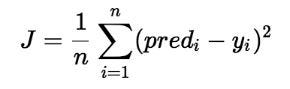
Here, n is the total number of data in the dataset.

You lot must be wondering where does the slope and intercept comes into play hither!!

          J = 1/n*sum(square(pred - y))          Which, can too exist written as :          J = 1/n*sum(foursquare(pred-(mx+b)))  i.due east, y = mx+b

Nosotros desire the Cost Role to be 0 or shut to zero,which is the all-time possible outcome i can get.
And how practise we acheive that?
Let'due south Look at the slope descent and how it helps improve the weights(m and b) to achieve the desired cost role.

Linear Regression with Gradient Descent

Gradient descent is an optimization algorithm used to find the values of parameters (coefficients) of a function that minimizes a cost function (cost).

To Read more almost it and get a perfect understanting of Gradient Descent i advise to read Jason Brownlee'south Web log.

To update chiliad and b values in order to reduce Price role (minimizing MSE value) and achieving the all-time fit line you can use the Gradient Descent. The idea is to start with random m and b values and and so iteratively updating the values, reaching minimum cost.

Steps followed by the Slope Descent to obtain lower cost function:

→ Initially,the values of m and b volition be 0 and the learning rate(α) will be introduced to the function.
The value of learning rate(α) is taken very small-scale,something between 0.01 or 0.0001.

The learning rate is a tuning parameter in an optimization algorithm that determines the pace size at each iteration while moving toward a minimum of a cost function.

→ Then the partial derivative is calculate for the cost function equation in terms of gradient(m) and also derivatives are calculated with respect to the intercept(b).After Adding the equation acheived will be.

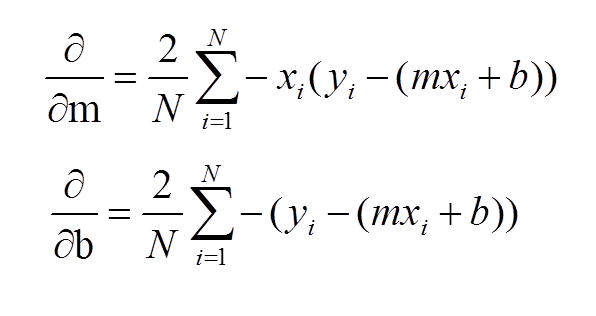
Guys familiar with Calculus will understand how the derivatives are taken.

If yous don't know calculus don't worry but understand how this works and information technology will exist more enough to recall intuitively what's happening behind the scenes and those who want to know the procedure of the derivation check out this blog by sebastian raschka.

→ Later the derivatives are calculated,The slope(m) and intercept(b) are updated with the help of the following equation.
m = m+α*derivative of grand
b = b+α*derivative of b
derivative of k and b are calculated above and α is the learning rate.

You must be wondering why I added and not subtracted,Well if you observe the outcome of the derivative you lot will see that the result is in negative.So the equation turns out to be :

one thousand = m — α*derivative of m

b = b — α*derivative of b

If you've gone through the Jason Brownlee'due south Weblog yous might have understood the intuition behind the gradient descent and how it tries to reach the global optima(Lowest price office value).

Why should we substract the weights(grand and b)with the derivative?
Gradient gives u.s.a. the direction of the steepest ascent of the loss function and the management of steepest descent is contrary to the gradient and that is why we substract the slope from the weights(m and b)

→ The process of updating the values of g and b continues until the toll office reaches the ideal value of 0 or close to 0.
The values of m and b at present will be the optimum value to describe the best fit line.

I hope things in a higher place are making sense to you.So,Now permit'south sympathize other important things related to the linear Regression.

Till now we accept understood How the Gradient(m) and Intercept(b) are calculated,what Price Part is and How Gradient Descent algorithm helps go the ideal Cost Function Value with the help of Simple Linear Regression.
For Multiple Linear Regression everything happens exactly same just the formula changes from a unproblematic equation to a bigger i as shown in a higher place.

Now to understand How Co-efficients are calculated in Multiple Linear Regression, please go to this link to get a cursory idea nigh it , Although you won't exist performing it manually ,but, it'south always good to know what's happening behind the scene.

Now Let's Await at how to check the quality of the model.

Interpreting the results of Linear Regression:

Photo past National Cancer Plant on Unsplash

You have cleaned the data and passed it on to the model,Now the question arises, How do y'all know if your Linear Regression Model is Performing well?

For That we Utilize the Statsmodel Bundle in Python and After plumbing equipment the data we do a .Summary() on the model,which gives result as shown in the motion picture beneath.(P.S. — I used a moving picture from google images)

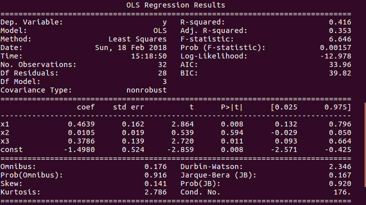
Now,If you Look at the Picture Advisedly you volition run across a bunch of different Statistical examination.
I Suppose you are familiar with R-Squared and Adjusted R-Squared shown on the top correct of the image,If yous don't no worries read my blog about R-Squared and P-value.

Here we will see what the lower cake of the image interprets.

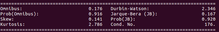
Omnibus/Prob(Bus):It is statistical test that tests the skewness and Kurtosis of the residuum.
A value of Charabanc shut to 0 show the normalcy(commonly distributed) of the residuals.
A value of Prob(Omnibus) close to 1 show the probability that the residuals are ordinarily distributed.
Skew: It is a measure of the symmetry of data,values closer to 0 indicates the residual distribution is normal.
Kurtosis: It is a measure of whether the data are heavy-tailed or lite-tailed relative to a normal distribution. That is, data sets with loftier kurtosis tend to accept heavy tails, or outliers. Data sets with depression kurtosis tend to accept light tails, or lack of outliers.
Greater Kurtosis tin exist interpreted as a tighter clustering of residuals around zero, implying a better model with few outliers.
Durbin-Watson:It is a statistical test to observe any auto-correlation at a lag 1 present in the residuals.
→ value of test is ever betwixt 0 and 4
→ IF value = 2 the there is no motorcar-correlation
→ IF value greater than(>) ii then there is negative automobile-correlation,which ways that the positive fault of one ascertainment increases the chance of negative error of another observation and vice versa.
→ IF value less than(<) ii the at that place is positive auto-correlation.
Jarque-Bera/Prob(Jarque-Bera):It is a Statistical exam which examination a goodness of fit of whether the sample data has skewness and kurtosis matching the normal distribution.
Prob(Jarque-Bera) indicates normality of the residuals.
Condition Number:This is a Statistical Test that measures the sensitivity of a function'due south output every bit compared to its input.
When there is multicollinearity present , nosotros can look much higher fluctuations to small changes in the data,So the value of the test volition be very loftier.
A lower value is expected,something below 30,or more specifically value closer to 1.

I hope this commodity helped yous understand the Algorithm and Near of the concepts related to it.
Coming up next Week,We will Sympathize the Logistic Regression.

HAPPY LEARNING!!!!!

Like my article? Do give me a clap and share it, as that will boost my conviction. Also, I post new articles every sun so stay connected for future articles of the nuts of data science and car learning series.

As well, do connect with me on LinkedIn.